module main
using Bcube
using LinearAlgebra
using StaticArrays
using DelimitedFiles
include(joinpath(@__DIR__, "..", "common", "common.jl"))
const eps_h = 1.0e-10
const hmin₀ = 1.e-8
const hmax₀ = 1.0e10
const DMPcurv₀ = 0.0
const wall_friction = false
@warn "wall friction is $(wall_friction)"
velocity(h, hu) = (hu * 2 * h) / (h * h + max(h * h, (3e-5)^2)) #desingularization
function _flux_HLL(qL, qR, n, flux, f_λ)
λL, λR = f_λ(qL), f_λ(qR)
λ⁻ = min(minimum(λL), minimum(λR), zero(λL[1]))
λ⁺ = max(maximum(λL), maximum(λR), zero(λL[1]))
function f_HLL(qL, qR, fL, fR)
if abs(λ⁺ - λ⁻) > 1.0e-12
fLn, fRn = dotn(fL, n), dotn(fR, n)
f = (λ⁺ * fLn - λ⁻ * fRn + λ⁻ * λ⁺ * (qR - qL)) / (λ⁺ - λ⁻)
else
f = 0.5 * (fL(qL) + fR(qR))
end
return f
end
map(f_HLL, qL, qR, flux(qL), flux(qR))
end
function shallow_water_maxeigval(q, gravity)
h, hu = q
u = velocity(h, hu)
return norm(u) + √(norm(gravity) * max(h, eps_h))
end
function shallow_water_maxeigval(q, n, gravity)
h, hu = q
un = velocity(h, hu) ⋅ n
return abs(un) + √(norm(gravity) * max(h, eps_h))
end
function shallow_water_eigval(q, n, gravity)
h, hu = q
un = velocity(h, hu) ⋅ n
c = √(norm(gravity) * max(h, eps_h))
return un - c, un + c
end
function compute_timestep!(q, mesh, dimcar, gn, CFL)
h, hu = q
degree = minimum(
feSpace -> get_degree(Bcube.get_function_space(feSpace)),
get_fespace.(get_fe_functions(q)),
)
λmax = var_on_centers(norm ∘ velocity(h, hu) + √(gn * h), mesh)
Δt = CFL * minimum(dimcar ./ λmax)
return Δt / (2degree + 1)
end
function flux_fitted(qi, qj, gni, gnj, Ri, Rj, φi, φj, nij, flux)
hj, huj = qj
_qj = (hj, Ri * huj)
φ_hi, φ_hui = φi
φ_hj, φ_huj = φj
δφ = (φ_hi - φ_hj, φ_hui - transpose(Rj) * φ_huj)
return flux(qi, _qj, gni, δφ, nij)
end
function flux_unfitted(qi, qj, gni, gnj, Pi, Pj, ℋi, ℋj, ϕi, ϕj, δφ, nij, flux)
_nij = inv(I - ϕi * ℋi) * Pi * nij
return flux(qi, qj, gni, δφ, _nij)
end
function flux_HLL(qi, qj, gni, δφ, nij)
δv_h, δv_hu = δφ
f_λ = x -> shallow_water_eigval(x, nij, gni)
flux = _flux_HLL(qi, qj, nij, y -> flux_sw(y, gni), f_λ)
flux_h, flux_hu = flux
return flux_h ⋅ δv_h + flux_hu ⋅ δv_hu
end
function _flux_HLL(qL, qR, n, flux, f_λ)
λL, λR = f_λ(qL), f_λ(qR)
λ⁻ = min(minimum(λL), minimum(λR), zero(λL[1]))
λ⁺ = max(maximum(λL), maximum(λR), zero(λL[1]))
function f_HLL(qL, qR, fL, fR)
fLn, fRn = dotn(fL, n), dotn(fR, n)
if abs(λ⁺ - λ⁻) > 1.0e-12
f = (λ⁺ * fLn - λ⁻ * fRn + λ⁻ * λ⁺ * (qR - qL)) / (λ⁺ - λ⁻)
else
f = 0.5 * (fLn + fRn)
end
return f
end
map(f_HLL, qL, qR, flux(qL), flux(qR))
end
function flux_sw(q, gn)
h, hu = q
u = velocity(h, hu)
huu = hu * transpose(u)
p_grav = 0.5 * gn * h * h
return h .* u, huu + p_grav * I
end
function apply_limitation!(q, params, cache)
h, hu = q
dΩ = params.dΩ
q_mean = Bcube.cell_mean(q, cache.cacheCellMean)
lim_h, h_proj = linear_scaling_limiter(
h,
dΩ;
bounds=(hmin₀, hmax₀),
DMPrelax=params.DMPrelax,
mass=cache.mass_sca,
)
set_dof_values!(h, get_dof_values(h_proj))
_, hu_mean, = q_mean
limited_var(a, a̅, lim_a) = a̅ + lim_a * (a - a̅)
projection_l2!(hu, limited_var(hu, hu_mean, lim_h), dΩ; mass=cache.mass_vec)
end
"""
Define closest point interpolator of a function f : here we cheat because we now the closest point on Gamma,
which is assumed to be a circle of radius 1 centered in (0,0)
"""
function closest_point_interp_func(pf, f)
return x -> begin
θ = atan(x[2], x[1])
Bcube.interpolate_at_point(pf, SA[cos(θ), sin(θ)], f...)
end
end
closest_point_interp = PhysicalFunction ∘ closest_point_interp_func
"""
Warning : only valid for P1 geometrical elements
"""
function fitted_closest_point_interp_func(pf, f)
return x -> begin
icell = Bcube.find_cell_index(pf, x)
cinfo = Bcube.CellInfo(pf.mesh, icell)
ctype = Bcube.celltype(cinfo)
@assert ctype isa Bcube.Bar2_t "not valid for elements different from P1"
A, B = Bcube.nodes(cinfo)
u = normalize(B.x - A.x)
l = (x - A.x) ⋅ u
H = A.x + l * u
y = Bcube.CellPoint(H, cinfo, Bcube.PhysicalDomain())
f_icell = Bcube.materialize(f, cinfo)
return Bcube.materialize(f_icell, y)
end
end
fitted_closest_point_interp = PhysicalFunction ∘ fitted_closest_point_interp_func
function unfitted_dg(;
mesh,
_ϕ,
h0,
u0,
g,
μ,
tfinal,
degree,
CFL,
flux,
Δt_min=0.0,
nitemax,
use_constant_Δt=false, # if true, a constant Δt is used
constant_Δt=0.0,
limitation=degree > 0,
)
(degree > 0 && !limitation) && @warn "degree > 0 but limitation disabled"
# Mesh
quad = Quadrature(QuadratureLobatto(), 2 * degree + 1)
dΩ = Measure(CellDomain(mesh), quad)
dΓ = Measure(InteriorFaceDomain(mesh), quad)
dΛ = Measure(BoundaryFaceDomain(mesh), quad)
nΓ = get_face_normals(dΓ)
nΛ = get_face_normals(dΛ)
dimcar = compute_dimcar(mesh)
# Projection material
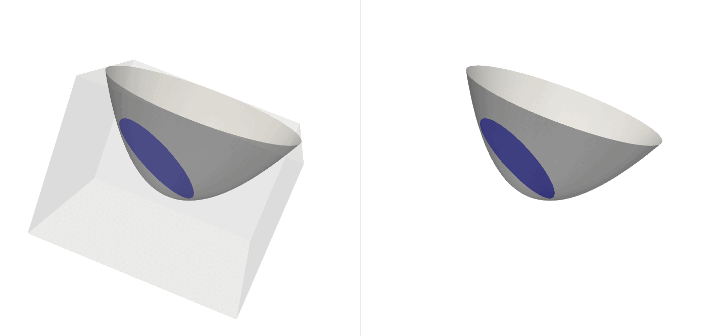
ϕ = PhysicalFunction(_ϕ)
ν = PhysicalFunction(x -> x ./ (norm(x) + 1e-20)) # analytic
H = PhysicalFunction(x -> 1 / (norm(x) + 1e-20)) # analytic
ℋ = PhysicalFunction(
x -> begin
x2 = x[1]^2
y2 = x[2]^2
return SA[
y2 (-x[1]*x[2])
(-x[1]*x[2]) x2
] ./ (x2 + y2)^(3 / 2)
end,
) # analytic
divℋ0 = PhysicalFunction(x -> -x ./ (norm(x) + 1e-20))
P = I - (ν ⊗ ν)
# FESpace
U_h = TrialFESpace(FunctionSpace(:Lagrange, degree), mesh, :discontinuous)
U_hu = TrialFESpace(
FunctionSpace(:Lagrange, degree),
mesh,
:discontinuous;
size=Bcube.spacedim(mesh),
)
V_h = TestFESpace(U_h)
V_hu = TestFESpace(U_hu)
U = MultiFESpace(U_h, U_hu)
V = MultiFESpace(V_h, V_hu)
# FEFunction
q = FEFunction(U)
projection_l2!(q, (h0, u0), mesh)
# Gravity op
gn = abs(g ⋅ ν)
# Flux
function flux_Γ(q, gn, P, ℋ, ϕ, φ, n)
flux_unfitted ∘ (
side⁻(q),
side⁺(q),
side⁻(gn),
side⁺(gn),
side⁻(P),
side⁺(P),
side⁻(ℋ),
side⁺(ℋ),
side⁻(ϕ),
side⁺(ϕ),
jump(φ),
side⁻(n),
flux,
)
end
function _flux_Λ(qi, closest_q, gni, Pi, ℋi, ϕi, φi, nij)
# Closest-point version
qg = closest_q
return flux_unfitted(qi, qg, gni, gni, Pi, Pi, ℋi, ℋi, ϕi, ϕi, φi, nij, flux)
end
function flux_Λ(q, closest_q, gn, P, ℋ, ϕ, φ, n)
_flux_Λ ∘ (
side⁻(q),
side⁻(closest_q),
side⁻(gn),
side⁻(P),
side⁻(ℋ),
side⁻(ϕ),
side⁻(φ),
side⁻(n),
)
end
function _flux_Ω(q, φ, ∇φ, gn, ν, P, ℋ, H, divℋ0, ϕ)
h, hu = q
u = hu / h
φh, φhu = φ
∇φh, ∇φhu = ∇φ
_q = (h, P * hu)
f_h, f_hu = flux_sw(_q, gn)
# Version Greer
Pg = inv(I - ϕ * ℋ) * P
∇Γ_φh = Pg * ∇φh # scalar version
∇Γ_φhu = ∇φhu * Pg # vector version
expr =
f_h ⋅ (∇Γ_φh - φh * (H * ν - ϕ * divℋ0)) +
f_hu ⊡ (∇Γ_φhu - φhu ⊗ (H * ν - ϕ * divℋ0))
if wall_friction
expr += -3μ * u / h ⋅ φhu
end
return expr
end
function flux_Ω(q, gn, P, ℋ, H, divℋ0, ϕ, φ)
_flux_Ω ∘ (q, φ, map(∇, φ), gn, ν, P, ℋ, H, divℋ0, ϕ)
end
# Rhs function
function compute_rhs!(rhs, qdofs)
_q = (FEFunction(U, qdofs)...,)
_closest_q = closest_point_interp(pf, _q)
function l(φ)
∫(flux_Ω(_q, gn, P, ℋ, H, divℋ0, ϕ, φ))dΩ -
∫(flux_Γ(_q, gn, P, ℋ, ϕ, φ, nΓ))dΓ -
∫(flux_Λ(_q, _closest_q, gn, P, ℋ, ϕ, φ, nΛ))dΛ
end
assemble_linear!(rhs, l, V)
end
function compute_rhs(qdofs)
rhs = zero(qdofs)
compute_rhs!(rhs, qdofs)
return rhs
end
# Mass matrix
m(q, φ) = ∫(q ⋅ φ)Measure(CellDomain(mesh), 2 * degree + 1) # whole domain
_M = assemble_bilinear(m, U, V)
M = factorize(_M)
# Limitation
if degree > 0
DMPrelax = DMPcurv₀ .* dimcar .^ 2
params = (; dΩ, DMPrelax)
cache = (
mass_sca=Bcube.build_mass_matrix(U_h, V_h, dΩ),
mass_vec=Bcube.build_mass_matrix(U_hu, V_hu, dΩ),
cacheCellMean=Bcube.build_cell_mean_cache(q, dΩ),
)
apply_limitation!(q, params, cache)
end
# Loop
t = 0.0
last_ite = false
rhs = Bcube.allocate_dofs(U)
qdofs = copy(get_dof_values(q))
for ite in 1:nitemax
Δt = if !use_constant_Δt
compute_timestep!(FEFunction(U, qdofs), mesh, dimcar, gn, CFL)
else
constant_Δt
end
Δt = max(Δt, Δt_min)
if Δt > tfinal - t
last_ite = true
Δt = tfinal - t
end
qdofs .= get_dof_values(q)
# udofs .= forward_euler(udofs, x -> M \ compute_rhs(x), Δt)
qdofs .= rk3_ssp(qdofs, x -> M \ compute_rhs(x), Δt)
t += Δt
set_dof_values!(q, qdofs)
limitation && apply_limitation!(q, params, cache)
last_ite && break
end
return (; q, pf)
end
function run_one_case()
# Settings
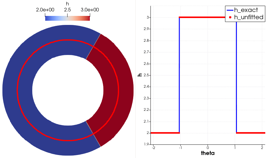
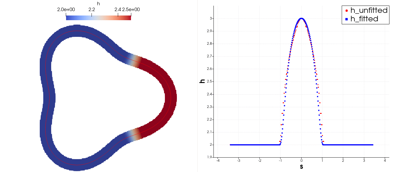
R = 1 # radius
CFL = 0.5
tfinal = 0.5
degree = 0
outdir = joinpath(@__DIR__, "tmp")
gn = 1.0
ϕmax = 0.3
n = 1024
mkpath(outdir)
# Initial solution / conditions
μ = 5.0
θc = 0.0
θlr = π / 3
hl0 = 3.0
hr0 = 2.0
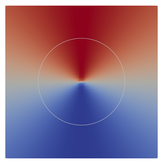
_θ(x) = atan(x[2], x[1])
u0 = PhysicalFunction(x -> @SVector zeros(Bcube.spacedim(mesh_fitted)))
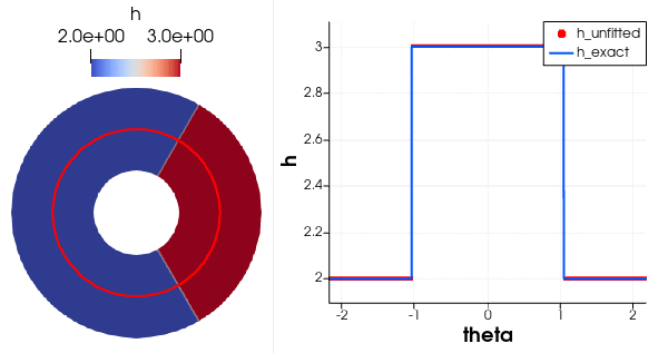
# h0 = PhysicalFunction(x -> abs(_θ(x) - θc) ≤ θlr ? hl0 : hr0)
h0 = PhysicalFunction(
x -> begin
__θ = _θ(x) - θc
if abs(__θ) ≤ θlr
return hr0 + (hl0 - hr0) * exp(1 / θlr^2) * exp(-1 / (θlr^2 - __θ^2)) # wrong
else
return hr0
end
end,
)
function _g(x)
if norm(x - xc) < 1e-9
return SA[0.0, 0.0] # no gravity vector on center
else
return gn * normalize(x - xc)
end
end
g = PhysicalFunction(_g)
# Unfitted solution
ϕ(x) = norm(x) - R # signed distance
l = 3R
## Mesh 1
println("UNFitted DG, n = $n, ϕmax = $ϕmax, degree = $degree")
mesh_unfitted =
rectangle_mesh(n, n; xmin=-l / 2, xmax=l / 2, ymin=-l / 2, ymax=l / 2)
indices = Bcube.identify_cells(mesh_unfitted, x -> abs(ϕ(x)) < ϕmax)
@assert length(indices) > 0 "no cell in clipped mesh" # the ϕmax is too harsh and there is no cell in the clipped mesh
mesh_unfitted = Bcube.domain_to_mesh(CellDomain(mesh_unfitted, indices))
if ncells(mesh_unfitted) <= 21 # check that all cells have at least one neighbor cell
c2c = Bcube.connectivity_cell2cell_by_faces(mesh_unfitted)
@assert c2c.minsize > 0 "disjoined cells"
end
sol_unfitted = unfitted_dg(;
mesh=mesh_unfitted,
_ϕ=ϕ,
h0,
u0,
g,
μ,
tfinal,
degree,
flux=flux_HLL,
CFL,
nitemax=typemax(Int),
Δt_min=0.0,
limitation=false,
use_constant_Δt=true,
constant_Δt=CFL * l / (n - 1) / √(gn * max(hl0, hr0)) / (2degree + 1),
)
end
run_one_case()
end